VLOOKUP vs. INDEX(MATCH) to look up related information
When working with spreadsheets it often happens that you want to look up related information that is already stored somewhere else, whether in the same spreadsheet or another one. There are several ways this can be done, but VLOOKUP (for vertical look up) and HLOOKUP (its horizontal lookup brother) are often the first ones people learn to use. Unfortunately, many stop there and do not learn a more powerful alternative.
Another option you should learn is the combination of two functions not directly designed for this (INDEX and MATCH) but which, when used together, can be more powerful than the familiar and fairly intuitive VLOOKUP function, especially in more complicated settings. Let’s look at some pros and cons of these different approaches.
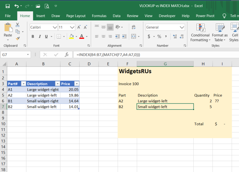
First, let’s look at a simple scenario and see how VLOOKUP can work for us. A company has a parts list and wants to use this to create an invoice, as in the screenshot below.

The syntax for VLOOKUP is as follows:
=VLOOKUP(what to lookup, where to look for it, column number to return value from, and (optional) approximate (TRUE) or exact (FALSE) match)
So in our example above, to look up the description for part A2 we would use the formula:
=VLOOKUP(F6,A4:C7,2,0,FALSE)
This in effect says: look up the exact part number found in cell F6 in the first column of the range A4:C7 and return the corresponding value from the second column of this range.

This is very helpful and works fine in many cases, but there are some significant limitations to keep in mind.
First, if we omit the optional, final parameter (or select TRUE, which is the default value if nothing is specified), our lookup range must be sorted alphabetically or numerically to find the correct value; if not, it will find the first one it thinks is close enough.
Second, the column to return must be to the right of the lookup column.
Third, you can only look up values in the first column of the specified range (which can become problematic if you are using named ranges).
Fourth, if you insert a column in your data table, you may be returning data from the wrong column (as your desired data may now be in column 3, not column 2). This limitation may also prevent you from getting the results you expect if you copy the formula to another column to use there.
In our simple example above, these considerations are easily met, but life isn’t always so simple. For more complicated scenarios the INDEX(MATCH) combination can be more forgiving. As mentioned above, while not designed for this purpose this is a good example of using a nested formula to accomplish something far more than the sum of its parts.
While not going into these functions individually in detail, here is the basic syntax needed:
=INDEX (value to return, (MATCH(value to look up, what to compare it against, type of match)))
For the next part# on the invoice, as in the screenshot below, the formula would be:
=INDEX(B4:B7,(MATCH(F7,A4:A7,0)))
This in effect says match exactly the part number in cell F7 to the list of part numbers in range A4:A7 and return the corresponding value in range B4:B7.

(For the type of match parameter, the options are 1=the largest value less than or equal to the lookup value, the lookup array must be in ascending order; 0=the first value that is exactly equal to the lookup value, the lookup array can be in any order, -1=the smallest value greater than or equal to the lookup value, the lookup array must be in descending order)
These advantages can become particularly important if the source table is large or complicated in nature.
It is worth noting here that since the formula uses ranges, it works in either a vertical or a horizontal direction and so can be used to replace both VLOOKUP and HLOOKUP.
Once you are comfortable working with nested formulas, either formula can be used to calculate the price, as in the screen shots below:


In the last formula (in I7), notice that the table references are used rather than the cell references. The advantage of doing this is that as new parts are added to the table they are automatically included in the formulas, which is a key advantage of using tables in such circumstances. However, that is a discussion for another day.
Don’t worry if you have to keep a cheat sheet handy to remember the syntax when using the Index(Match) option; many of us do. Its benefits, though, make it worth looking up the syntax as needed.
Finally, it should be noted that in the fall of 2019 Microsoft added a new function called XLOOKUP in Office 365 that replaces HLOOKUP and VLOOKUP and has the same advantages of the INDEX(MATCH) formula. It is expected that this will eventually move into all newer versions of Excel.


Pingback: Multiple Criteria Lookup Formula, Or How To Create Complicated Formulas When Required - Sparrowsolutions.ca